Racism

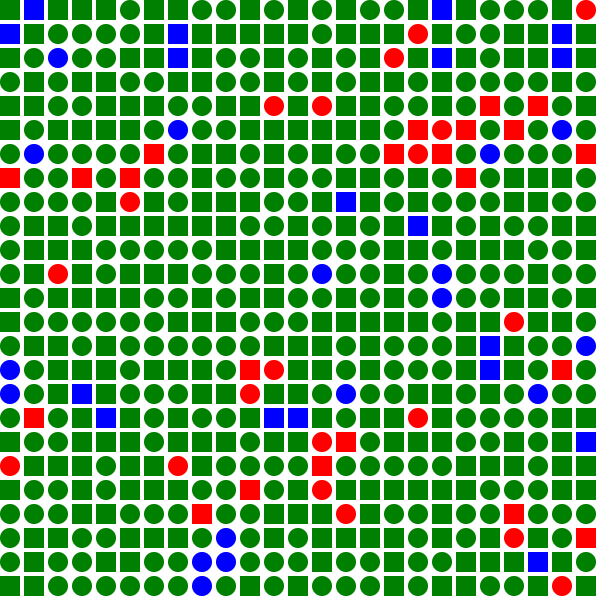
An initial population of two groups: square and circle. Green squares are happy (they have at least one neighbour who is the same color), blue squares are entirely surrounded by shapes like them and only red shapes are alone.
Stats: happy: 583; among equals: 35.

(Fair warning: the following deals with racism in modelled groups; solutions for intervention in Real Life are out of scope of this post, as I do not have relevant experience. Also if you generalize the real world from a double array of boolean variables I don’t want to know you.)

What can a computer model tell us about racism?

Well this blog post mentions an interesting model Thomas Schelling made: if you start with a grid of two different types (in this case circles and squares) and then randomly swap unhappy pieces (pieces are unhappy if there are not some minimum number of its neighbours that are the same type as it) you will end up with a completely segregated board.

This apparently surprised Schelling and has been used as an argument for why even not-racists societies must be intervened in, lets they produce a racists outcome.

Personally I think that is bunk and is just the logical result of a relatively simple (and innocent) misunderstanding and in this blog post intend to show how and how to fix it.

In the first figure I have a randomly created initial community of squares and circles, 25 by 25 (625 in total). The requirement for happiness is simple: a piece is happy so long as it is not alone. In other words as long as one neighbour is the same type as it is happy. The reason I choose this is simple: if this arrangement reliably comes out segregated then there is no point in making the happiness requirement higher.

We will have shown that any preference at all will give a segregated outcome (pedantic point: the segregated outcome is trivial in the case where the pieces require as many neighbours to be of its own type as there are neighbours and the case where the pieces have no preference is stable in its initial configuration and thus the outcome will be completely random. Therefore the point at which the board ends up segregated will be somewhere between these two points).

As you can see in the caption in this configuration even a completely random board has 583 happy pieces (93.28% of the total) and 35 pieces that have neighbours that are entirely the same type as it (5.6%). Since each piece has 4 neighbours (we count only direct neighbours) that means a piece has a (or 93.75%) chance of being happy and a 6.25% chance of being completely surrounded by pieces of the opposite type (it also has a 6.25% chance of being completely surrounded by pieces of the same type, but not without being happy, which means it is included in the 6.25% chance).

So our initial numbers look spot on. The number of squares that are among equals is a bit on the low side, but nothing unreasonable.

Now that we have a way to produce the initial version, lets look at getting to the next generation. There are a bunch of different ways to swap pieces, so our first attempt will be one that saves time by only swapping pieces that are unhappy and only swapping them with pieces of the opposite type (since a piece of the same type would by definition be unhappy at the same position too). If we don’t have an unhappy piece of the opposite type, we randomly select any piece with that type.
When there are no pieces that are unhappy we don’t swap any.

Next we need a way to measure how segregated a board is. This is important because on a big enough board (and as you can see the boards we are working with are plenty big enough) there will, by purely random chance, be some portions of the board that are very segregated. Humans are really really good at seeing patterns, so good in fact that we can see patterns that just aren’t there.

There is a statistical distribution that models such things – as long as each occurrence is random and independent of the others the Poisson distribution can describe exactly how it should behave, including how often we should see any given number of consecutive pieces of the same type. Unfortunately this is quite a bit more statistics that I understand, so what I will just do is look at how many pieces are among equals – that is each of their neighbours is of the same type.

As a test I made a simulation that ran over ten randomly generated boards, printed how many pieces were happy and how many were among equals and then randomly swap all the unhappy pieces with other pieces. We do this for ten iterations (per board).

That was at least the plan. As it turns out those boards usually ends up in a stable configuration (that is no pieces are moved), but where some of the pieces are still not happy.

I wrote a more complicated swap algorithm, which sorts the two pieces types into two separate lists, then fill which ever list is shortest with randomly chosen pieces of the same type from the board. Then the two lists are shuffled and the pieces are swapped with a piece of the opposite type. This works, because now any piece is unlikely to be swapped same piece more than once.

This algorithm appears to terminate very fast, typically before the 6th iteration, and can only fail to swap an unhappy piece in the extreme case that there are fewer pieces of the opposite type on the entire board than there are unhappy pieces of this type.

For each of the boards the algorithm had terminated with no unhappy pieces after ten iterations. Since the requirement for happiness was just one neighbour like it self, most of the pieces were happy from the beginning and therefore had little chance to be moved.

Initially there were an average of 584.73 happy pieces (std deviation of 7.23). 38.91 pieces are surrounded entirely by pieces of the same type (std deviation of 8.14). After this every piece is happy (625, std deviation 0) and 92.55 pieces are surrounded entirely by pieces of the same type (std deviation 17.42). This is statistically very significant (p <= 0.0021) and causal.

So yes, just that simple change means the neighbourhoods are now more segregated. Okay no big surprise, in fact anything else would have been. Lets try making the pieces more racist by upgrading the happiness requirement to a minimum of 3 neighbours of the same type.

Unfortunately we will have to use a new strategy because the previous strategy results in fewer happy pieces — since there are so few happy pieces we are more likely to randomly move them to a new place (where they won’t be happy) than to move an unhappy piece to a place where it will be happy.

Instead we will only move a limited number of pieces of each type (in this case 10). Unfortunately this requires far more iterations, whereas before we could be happy with 10 and terminated well before that, we now have to spend 500 iterations and even then not all the pieces are happy.

Still the initial assumption held up: On average 194.73 pieces are happy initially (std deviation 15.79), 38.55 are among equals (std deviation 8.51). After the algorithm has run the board looks very different: Unlike the previous runs not every piece is happy, but on average 585.18 are (std 16.99). However fully 492.09 are, on average, among equals (std deviation 32.49). This is an incredible 13.96 sigmas above the previous mean.

Hopefully this proves the point: if the pieces are moved such that they are even slightly biased towards their own type, we get overall a statistically significantly more segregated board. If we make them more biased we end up with a board that is segregated to an almost unbelievable degree. 13.96 sigma!

Why? Well remember that we are more likely to move pieces that are not happy than happy pieces and if we have, by random chance, an arrangement like this: (on a 3×3 board) XXX XOX XXX Then the O will be unhappy (in the first case) unless either of the happy Xs are replaced with an O, but if it is swapped (which will most likely be with an X) then that entire block will be segregated, and the O has a of being put in a place where it is now happy – likely in its own cluster.

With a happiness requirement of 1 similar neighbour it is perfectly possible to arrange the board such that every piece is happy, but there are no clusters (just put each piece next to one and only one piece of its own type) but this is exceptionally unlikely to just happen by chance.

To sum up, here is what we have shown so far: first that if you introduce a slight bias you get a segregated board, that if you make this bias larger you get a board that is far more segregated and that finally this is because happy pieces are more likely to happen in clusters, so when we move the pieces around we are more likely to stop moving them if they are in a cluster.

Now what to do about it? Some suggests that this proves the system needs outside interference, but I think it is a flaw in how this system models the world: our system doesn’t take into account peoples preference for new things: we don’t want to eat the same thing every day (almost no matter how much we like it), we want to see new movies, etc.

My hypotheses is that if we change the happiness function such that the pieces are happy when they have at least one neighbour that is the opposite type of this piece (in addition to 2 pieces that are the same type) then, even if not all the pieces are happy, we will get a board that is far less segregated, perhaps even less segregated than the initial random board.

My claim is that this model more accurately describes reality (to the extend a 25×25 board can ever really describe such a complex issue as racism).

Now that we have a hypothesis, lets test it.

Here is what a typical board looked like (I have changed the rendering code since the first picture, which is why this looks somewhat different):

However the colors confuse this a bit so lets look at the same example, but this time recolored for the type of the piece, rather than its happiness.

Now lets compare this to the situation where the pieces only have a minimum requirement of two similar neighbors, but no requirement or penalty for having an opposite type neighbor:

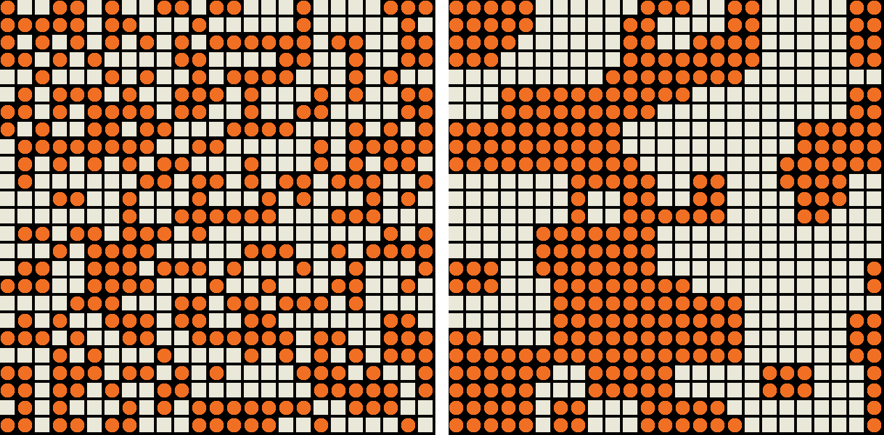
The board when the pieces have no other type requirements, colored for types.

</div>

Holy gentrification, batman – and the numbers show it too, after 500 iterations on average 259.27 pieces are entirely among equals (std dev 28.78), which is 7.72 sigmas above the mean, and statistically significant at p < 0.0001.

In contrasts the numbers are much different for case where the pieces wants just one neighbour of the opposite type, only 518.73 are happy (std dev 42.55) compared to the previous case where all pieces were happy, but also only 20.72 are among equals (std dev 10.23), which is only 0.24 sigmas above the mean which is not statistically significant (that is it could easily just be random).

I am not happy with an inconclusive result, so lets run just this simulation with 100 boards. In this case 46.69 are among equals (std dev 9.53) with a z score (that is, number of sigmas above average) of 0.70, which is still not statistically significant but we are at least getting closer, which suggest there is an effect, but that it is very, very small.

Since among equals isn’t a perfect measure of gentrification and the boards are very nicely separated when we look at them, I hope this satisfy most of you that a preference for new things can remove the need for interference without producing much gentrification and that this is a more correct model of reality than assuming we only have in-group preferences.

There are lots and lots of variations one could make based on this board model – what would happen if, for example, the pieces had different requirements for happiness? Would we finally get a statistically significantly more segregated boards if I ran the simulation with a thousand boards? What if types weren’t binary, but continuos? What if there were more than one type? What if etc.

If you come up with a simulation for either, please post a link in the comments (if you want a copy of my data, email me as I haven’t really found a good way to format them for the web yet).

Edit: 7th of August. It turns out Schelling was wrong about his model)