Zipfs law
Recently I have been reading Christian Rudders book Dataclysm, and in it he mentions a very interesting result: If you rank all the words in a text and then multiply the rank of each word by how often it occurs what you get is, approximately, a constant.
This is just another way of saying that the second most commonly used word is used only half as many times as the most common word, the third most commonly used word is used only one third as often, etc.
I want to test this theory out, but first we need some text with a lot of words (because like anything statistical the higher N we use the better our results are going to be) and, if possible, written by just one person so that we don’t end up just getting the average use of words over a group of people.
Fortunately Project Gutenberg has Saint Thomas Aquinas Summa Theologica which is both written by one person and sufficiently huge (2.8 megabyte of raw text! And that is only part one) that we should be able to get some good results from it.
Running a simple python script that I totally didn’t have to spend 2 hours writing gives these numbers as the ten most common:
- the 37221
- of 19320
- is 17165
- to 13748
- in 11714
- and 9220
- as 8084
- that 7842
- a 6538
- not 645
That seems reasonable, so lets insert the graph for Zipfs distribution:
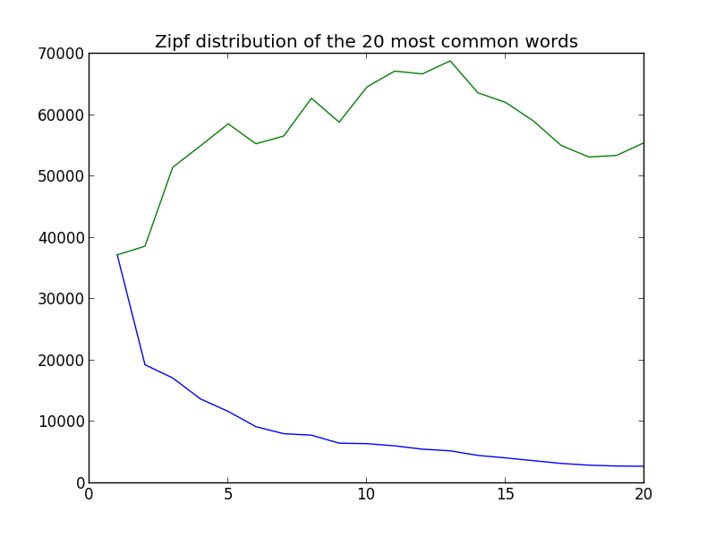 The green line is the zipf distribution, the blue line is how often the words are used.
We expected a mostly straight line and instead we got a very ragged green line that doesn’t follow what we want – but lets try one more time with the 1000 most common words:
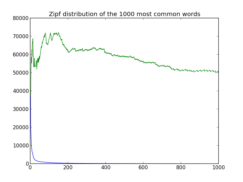
Argg, that is no good. Yes it starts to stabilize at around 200 words, but look at the blue line — we have reached the long tail of words were we expect the text to not be in-line with the distribution the: 200th most common word (love) is only in the text 307 times, whereas the the 10th most common word (not) is in the text 6459 times.
If we take a look at the fifty most common words we can start to see some issues:
17) Obj. 3238 (55046) 18) God 2954 (53172) 19) but 2812 (53428) 21) But 2764 (58044)
Yes, I forgot to remove the punctuation and make all the words lower case. Lets fix that (and also remove any words that are now of length zero, because they were never words in the first place):
So the new list of the twenty most common words is:
- the 39029
- of 19661
- is 17905
- to 14020
- in 12530
- and 9855
- that 8675
- as 8550
- it 7676
- a 7629
- not 6707
- but 5650
- by 5632
- be 5503
- god 4852
- are 4702
- for 4443
- which 4255
- from 3800
- things 3492
And in graph form:
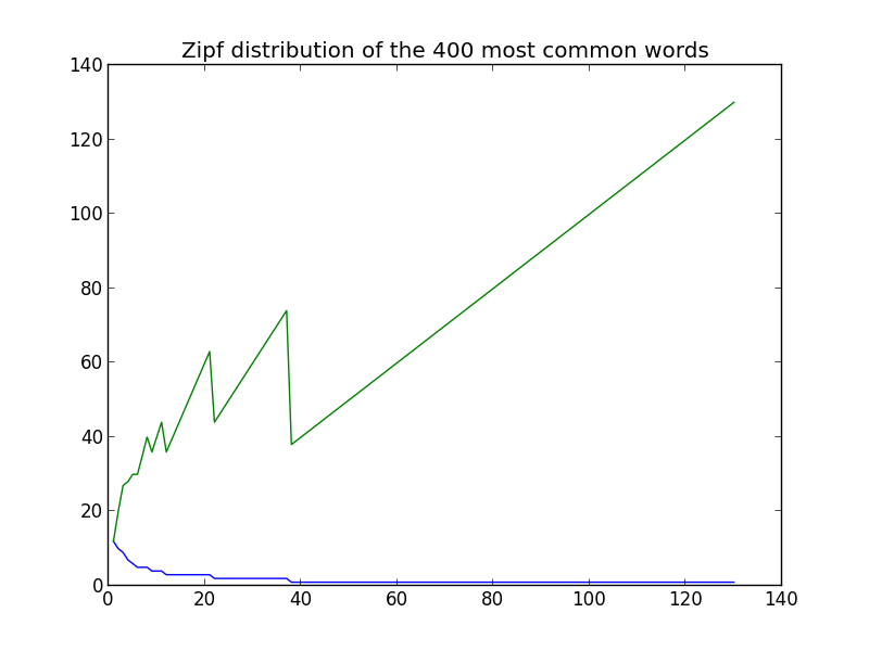
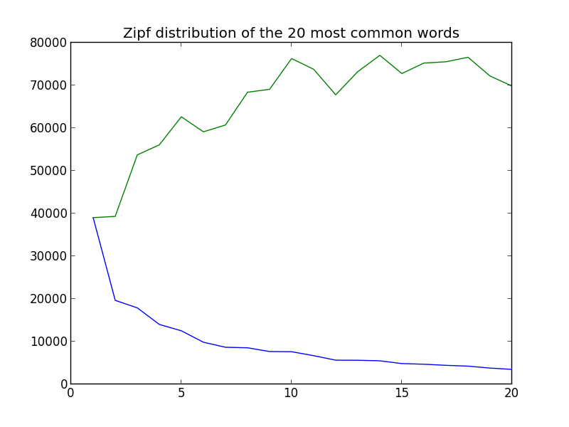 The tail of what we show here is now closer to what we expect but the graph is still not close enough, so lets look at the 400 most common words:
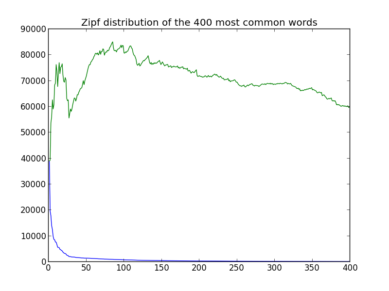 This isn’t completely what we expected, but unlike before it doesn’t seem that much of either – there are some outliers (especially the first few words which is what we would expect since their relative rank changes the most) but the output averages around a straight line fairly well.
First we tried with a really large text, lets try again with a much shorter text. In this case we will use the declaration of independence (available here) which is 1335 words long (Summa is 504243 words long, that is more than half a million words).
The top ten words are:
- the 39029 (39029)
- of 19661 (39322)
- is 17905 (53715)
- to 14020 (56080)
- in 12530 (62650)
- and 9855 (59130)
- that 8675 (60725)
- as 8550 (68400)
- it 7676 (69084)
- a 7629 (76290)
And the graph: 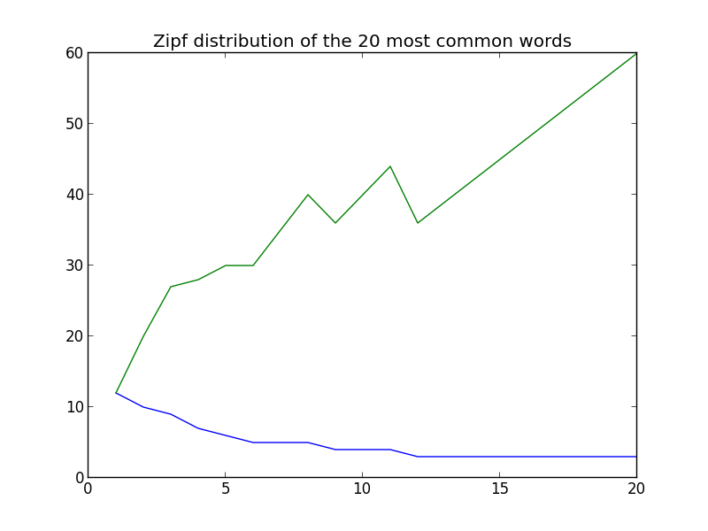
Once again we get that unsatisfying not quite what we were expecting result (we can disregard everything after the 12th or so word, at that point the words aren’t repeated enough to matter).
We really didn’t have enough data to do this, but here is the algorithm running on my python source code:
And the 10 most common words:
- count 12
- idx 10
- def 9
- word 7
- for 6
- return 5
- import 5
- in 5
- d 4
- enumeration 4
That is almost exactly what we would expect when we don’t have enough data.
I am really surprised that we didn’t see a stronger Zipf’s distribution for the text. We did everything right, it was huge, it was human made, etc. Most likely there is still some bugs in my code that lowers the word count of some of the words by interpretating what should have been the same word as two (or more) different words because they are written slightly differently.
Which means I will have to come back to this subject later.